Tracking with manually annotated edges
One important feature of LapTrack is tracking particles with preserving the ground-truth (for example manually annotated) point-to-point connections. This notebooks demonstrates its example usage with napari.
[ ]:
%pip install -q --upgrade -r requirements.txt
Importing packages
[1]:
import napari
import numpy as np
import pandas as pd
import json
from IPython.display import display
from skimage.io import imread
from skimage.measure import regionprops_table
from matplotlib import pyplot as plt

from laptrack import LapTrack
Loading data
Load images and show them in the viewer.
[2]:
images = imread("napari_interactive_fix_data/example_images.tif")
labels = imread("napari_interactive_fix_data/example_label.tif")
[3]:
viewer = napari.Viewer()
viewer.add_image(images, name="images")
viewer.add_labels(labels, name="labels")
original_camera_state = viewer.camera.dict()
with open("napari_interactive_fix_data/camera_state.json", "r") as f:
    camera_state = json.load(f)
Calculating centroids of the segmentation
Calculate centroids of each segmentation by regionprops_table.
[4]:
def calc_frame_regionprops(labels):  # noqa: E302
    dfs = []
    for frame in range(labels.shape[0]):
        df = pd.DataFrame(
            regionprops_table(labels[frame], properties=["label", "centroid"])
        )
        df["frame"] = frame
        dfs.append(df)
    return pd.concat(dfs)


regionprops_df = calc_frame_regionprops(labels)
display(regionprops_df.head())
| label | centroid-0 | centroid-1 | frame | |
|---|---|---|---|---|
| 0 | 3 | 103.091603 | 195.816794 | 0 |
| 1 | 25 | 151.812048 | 15.674699 | 0 |
| 2 | 35 | 31.552063 | 43.740668 | 0 |
| 3 | 59 | 60.389432 | 76.156556 | 0 |
| 4 | 64 | 125.100457 | 21.646119 | 0 |
Tracking by LapTrack
Tracking the centroids using the default sqeuclidean metric.
[5]:
lt = LapTrack(track_cost_cutoff=100**2, splitting_cost_cutoff=20**2)
track_df, split_df, _ = lt.predict_dataframe(
    regionprops_df,
    coordinate_cols=["centroid-0", "centroid-1"],
    only_coordinate_cols=False,
)
track_df.head()
[5]:
| label | centroid-0 | centroid-1 | frame_y | tree_id | track_id | ||
|---|---|---|---|---|---|---|---|
| frame | index | ||||||
| 0 | 0 | 3 | 103.091603 | 195.816794 | 0 | 0 | 0 |
| 1 | 25 | 151.812048 | 15.674699 | 0 | 1 | 1 | |
| 2 | 35 | 31.552063 | 43.740668 | 0 | 2 | 2 | |
| 3 | 59 | 60.389432 | 76.156556 | 0 | 3 | 3 | |
| 4 | 64 | 125.100457 | 21.646119 | 0 | 4 | 4 |
Adding the tracked data to the viewer
Display the tracking results. The objects with the same track_id is shown by the same label.
[6]:
track_label_image = np.zeros_like(labels)
for (frame, _), row in track_df.iterrows():
    track_label_image[frame][labels[frame] == row["label"]] = row["track_id"] + 1
[7]:
viewer.layers["labels"].visible = False
viewer.add_labels(track_label_image)
[7]:
<Labels layer 'track_label_image' at 0x1800c6a70>
Take screenshot of currente state
[8]:
plt.figure(figsize=(6, 3))
viewer.camera.update(camera_state)
viewer.dims.current_step = (1, 0, 0)
screenshot_before1 = viewer.screenshot()
viewer.dims.current_step = (2, 0, 0)
screenshot_before2 = viewer.screenshot()
viewer.camera.update(original_camera_state)
<Figure size 600x300 with 0 Axes>
Manual correction
Manually annotate a correct track by placing points using the Points layer.
Here, this step is emurated by loading the data to the layer.
[9]:
manual_corrected = np.load("napari_interactive_fix_data/manual_corrected.npy")
viewer.add_points(
    manual_corrected, name="manually_validated_tracks", size=10, face_color="red"
)
[9]:
<Points layer 'manually_validated_tracks' at 0x181b93520>
Loading manually annotated data
The data from the Points layer and the Labels layer are loaded to get the updated segmentation and annotation results.
[10]:
manual_corrected = viewer.layers["manually_validated_tracks"].data.astype(np.int16)
# you can also redraw the labels
new_labels = viewer.layers["track_label_image"].data
# get label values at the placed points
validated_track_labels = new_labels[tuple(manual_corrected.T)]
validated_frames = manual_corrected[:, 0]
again calculate the centroids of the segmentation
[11]:
new_regionprops_df = calc_frame_regionprops(new_labels).reset_index(drop=True)
new_regionprops_df.head()
[11]:
| label | centroid-0 | centroid-1 | frame | |
|---|---|---|---|---|
| 0 | 1 | 103.091603 | 195.816794 | 0 |
| 1 | 2 | 151.812048 | 15.674699 | 0 |
| 2 | 3 | 31.552063 | 43.740668 | 0 |
| 3 | 4 | 60.389432 | 76.156556 | 0 |
| 4 | 5 | 125.100457 | 21.646119 | 0 |
[12]:
validated_points = np.array(list(zip(validated_frames, validated_track_labels)))
validated_points = validated_points[np.argsort(validated_points[:, 0])]
print(validated_points)
[[ 0 34]
 [ 1 34]
 [ 2  6]
 [ 3  4]
 [ 4  9]
 [ 5  9]]
Eet the validated edges (track assigments) in terms of the iloc of the dataframe (making use of the index this time).
validated_point_iloc_pairs is the pairs of the ilocs of the validated points
[13]:
def get_iloc(frame, label):
    df = new_regionprops_df[
        (new_regionprops_df["frame"] == frame) & (new_regionprops_df["label"] == label)
    ]
    assert len(df) == 1
    return df.iloc[0].name


validated_point_ilocs = [get_iloc(frame, label) for frame, label in validated_points]
validated_point_iloc_pairs = list(
    zip(validated_point_ilocs[:-1], validated_point_ilocs[1:])
)
print(validated_point_iloc_pairs)
display(new_regionprops_df.iloc[validated_point_ilocs])
[(33, 69), (69, 88), (88, 132), (132, 182), (182, 230)]
| label | centroid-0 | centroid-1 | frame | |
|---|---|---|---|---|
| 33 | 34 | 108.448276 | 108.586207 | 0 |
| 69 | 34 | 92.097561 | 112.112805 | 1 |
| 88 | 6 | 68.569405 | 116.014164 | 2 |
| 132 | 4 | 52.942993 | 114.076010 | 3 |
| 182 | 9 | 36.493888 | 117.039120 | 4 |
| 230 | 9 | 41.824363 | 113.631728 | 5 |
Second tracking preserving manually corrected data
This is the core of this example: we can track the centroids again with preserving the annotation (connected_edges).
[14]:
lt = LapTrack(track_cost_cutoff=100**2, splitting_cost_cutoff=20**2)
new_track_df, _new_split_df, _ = lt.predict_dataframe(
    new_regionprops_df,
    coordinate_cols=["centroid-0", "centroid-1"],
    only_coordinate_cols=False,
    connected_edges=validated_point_iloc_pairs,
)
[15]:
new_track_df
[15]:
| label | centroid-0 | centroid-1 | frame_y | tree_id | track_id | ||
|---|---|---|---|---|---|---|---|
| frame | index | ||||||
| 0 | 0 | 1 | 103.091603 | 195.816794 | 0 | 0 | 0 |
| 1 | 2 | 151.812048 | 15.674699 | 0 | 1 | 1 | |
| 2 | 3 | 31.552063 | 43.740668 | 0 | 2 | 2 | |
| 3 | 4 | 60.389432 | 76.156556 | 0 | 3 | 3 | |
| 4 | 5 | 125.100457 | 21.646119 | 0 | 4 | 4 | |
| ... | ... | ... | ... | ... | ... | ... | ... |
| 5 | 45 | 55 | 95.888179 | 48.552716 | 5 | 42 | 54 |
| 46 | 56 | 188.176301 | 71.471098 | 5 | 38 | 55 | |
| 47 | 57 | 20.024096 | 196.915663 | 5 | 11 | 56 | |
| 48 | 58 | 193.452991 | 89.854701 | 5 | 38 | 57 | |
| 49 | 59 | 4.693182 | 191.176136 | 5 | 11 | 58 |
273 rows × 6 columns
Adding updated data to viewer
Display the updated tracking results. The objects with the same track_id is shown by the same label.
[16]:
new_track_label_image = np.zeros_like(new_labels)
for (frame, _), row in new_track_df.iterrows():
    new_track_label_image[frame][new_labels[frame] == row["label"]] = (
        row["track_id"] + 1
    )
viewer.layers["track_label_image"].visible = False
viewer.add_labels(new_track_label_image)
[16]:
<Labels layer 'new_track_label_image' at 0x160c9bc40>
Take screenshots
(the following codes exist to take screenshots of the viewer for the thumbnail.)
[17]:
plt.figure(figsize=(6, 3))
viewer.camera.update(camera_state)
<Figure size 600x300 with 0 Axes>
[18]:
plt.figure(figsize=(6, 3))
viewer.layers.move_multiple([3], 5)
viewer.camera.update(camera_state)
viewer.dims.current_step = (1, 0, 0)
screenshot_after1 = viewer.screenshot()
viewer.dims.current_step = (2, 0, 0)
screenshot_after2 = viewer.screenshot()
viewer.camera.update(original_camera_state)
<Figure size 600x300 with 0 Axes>
[20]:
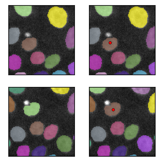
fig, axes = plt.subplots(2, 2, figsize=(3, 3))
screenshots = [
    screenshot_before1,
    screenshot_before2,
    screenshot_after1,
    screenshot_after2,
]
for ax, img in zip(np.ravel(axes.T), screenshots):
    ax.imshow(img)
    ax.set_xticks([])
    ax.set_yticks([])
fig.tight_layout()
[22]:
# camera_state = viewer.camera.dict()
# with open("napari_interactive_fix_data/camera_state.json","w") as f:
#     json.dump(camera_state,f)