Core tracking API by examples

This notebook illustrates the use of core APIs with a simple example.

try:
    import google.colab

    %pip install -q --upgrade laptrack matplotlib spacy flask pandas
    # upgrade packages to avoid pip warnings if the notebook is run in colab
except:
    %pip install -q --upgrade laptrack matplotlib pandas

Note: you may need to restart the kernel to use updated packages.

Note: Restart the runtime when you are on Google Colab and you see an error in matplotlib.

Importing packages

laptrack.LapTrack is the core object for tracking.

from os import path
import pandas as pd
from IPython.display import display
from matplotlib import pyplot as plt
from laptrack import LapTrack
from laptrack import datasets

plt.rcParams["font.family"] = ""

Matplotlib is building the font cache; this may take a moment.

Loading data

Load the example point coordinates from a CSV file.

spots_df has columns ["frame", "position_x", "position_y"] (can be arbitrary, and the column names for tracking will be specified later).

spots_df = datasets.simple_tracks()
display(spots_df.head())

Downloading file 'sample_data.csv' from 'https://raw.githubusercontent.com/yfukai/laptrack/97943e8b61a5fa6e9cdabf2968037c4b1f8cbf32/docs/examples/sample_data.csv' to '/home/docs/.cache/laptrack'.

	frame	position_x	position_y
0	0	178.412575	185.188661
1	1	236.963642	219.971473
2	1	185.175899	185.188661
3	2	190.006845	182.483331
4	2	190.200083	188.280466

Tracking

Initializing LapTrack object

First, initialize the LapTrack object with parameters.

max_distance = 15
lt = LapTrack(
    track_dist_metric="sqeuclidean",  # The similarity metric for particles. See `scipy.spatial.distance.cdist` for allowed values.
    splitting_dist_metric="sqeuclidean",
    merging_dist_metric="sqeuclidean",
    # the square of the cutoff distance for the "sqeuclidean" metric
    track_cost_cutoff=max_distance**2,
    splitting_cost_cutoff=max_distance**2,  # or False for non-splitting case
    merging_cost_cutoff=max_distance**2,  # or False for non-merging case
)

Example 1: using predict_dataframe to track pandas DataFrame coordinates

predict_dataframe is the easiest option when you have the coordinate data in pandas DataFrame.

track_df, split_df, merge_df = lt.predict_dataframe(
    spots_df,
    coordinate_cols=[
        "position_x",
        "position_y",
    ],  # the column names for the coordinates
    frame_col="frame",  # the column name for the frame (default "frame")
    only_coordinate_cols=False,  # if False, returned track_df includes columns not in coordinate_cols.
    # False will be the default in the major release.
)

track_df is the original dataframe with additional columns “track_id” and “tree_id”.

The track_id is a unique id for each track segments without branches. A new id is assigned when a splitting and merging occured.

The tree_id is a unique id for each “clonal” tracks sharing the same ancestor.

keys = ["position_x", "position_y", "track_id", "tree_id"]
display(track_df[keys].head())

		position_x	position_y	track_id	tree_id
frame	index
0	0	178.412575	185.188661	0	0
1	0	236.963642	219.971473	1	1
	1	185.175899	185.188661	0	0
2	0	190.006845	182.483331	2	0
	1	190.200083	188.280466	3	0

split_df is a dataframe for splitting events with the following columns: - “parent_track_id” : the track id of the parent - “child_track_id” : the track id of the parent

display(split_df)

	parent_track_id	child_track_id
0	0	2
1	0	3

merge_df is a dataframe for merging events with the following columns: - “parent_track_id” : the track id of the parent - “child_track_id” : the track id of the parent

display(merge_df)

	parent_track_id	child_track_id
0	3	5
1	4	5

We can display tracks in napari as follows:

# Does not work in Colab
#
# import napari
# v = napari.Viewer()
# v.add_points(spots_df[["frame", "position_x", "position_y"]])
# track_df2 = track_df.reset_index()
# v.add_tracks(track_df2[["track_id", "frame", "position_x", "position_y"]])

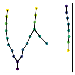
Plotting tracks in matplotlib

plt.figure(figsize=(3, 3))
frames = track_df.index.get_level_values("frame")
frame_range = [frames.min(), frames.max()]
k1, k2 = "position_y", "position_x"
keys = [k1, k2]


def get_track_end(track_id, first=True):
    df = track_df[track_df["track_id"] == track_id].sort_index(level="frame")
    return df.iloc[0 if first else -1][keys]


for track_id, grp in track_df.groupby("track_id"):
    df = grp.reset_index().sort_values("frame")
    plt.scatter(df[k1], df[k2], c=df["frame"], vmin=frame_range[0], vmax=frame_range[1])
    for i in range(len(df) - 1):
        pos1 = df.iloc[i][keys]
        pos2 = df.iloc[i + 1][keys]
        plt.plot([pos1[0], pos2[0]], [pos1[1], pos2[1]], "-k")
    for _, row in list(split_df.iterrows()) + list(merge_df.iterrows()):
        pos1 = get_track_end(row["parent_track_id"], first=False)
        pos2 = get_track_end(row["child_track_id"], first=True)
        plt.plot([pos1[0], pos2[0]], [pos1[1], pos2[1]], "-k")


plt.xticks([])
plt.yticks([])

([], [])

Example 2: using predict to track frame-wise-organized coordinates to make networkx tree

predict_dataframe is a thin wrapper of the predict function, the core tracking function of the LapTrack object.

One can directly use this function with the input of the frame-wise coordinate list and the output of networkx DiGraph object representing the lineage tree.

frame_max = spots_df["frame"].max()
coords = []
for i in range(frame_max):
    df = spots_df[spots_df["frame"] == i]
    coords.append(df[["position_x", "position_y"]].values)

The input variable coords should be organized as the frame-wise list of the point coordinates.

The coordinate dimension is (particle, dimension).

display(coords[:5])

[array([[178.41257464, 185.18866074]]),
 array([[236.9636424 , 219.97147327],
        [185.1758993 , 185.18866074]]),
 array([[190.00684549, 182.48333087],
        [190.20008333, 188.2804663 ],
        [230.97326914, 220.16471112]]),
 array([[195.61074306, 181.32390379],
        [196.1904566 , 189.05341768],
        [225.75584726, 220.74442466]]),
 array([[200.82816494, 178.81181177],
        [201.79435418, 191.9519854 ],
        [201.98759203, 206.05834826],
        [219.95871183, 221.51737605]])]

predict function generates a networkx DiGraph object from the coordinates

track_tree = lt.predict(
    coords,
)

The returned track_tree is the connection between spots, represented as ((frame1,index1), (frame2,index2)) …

For example, ((0, 0), (1, 1)) means the connection between [178.41257464, 185.18866074] and [185.1758993 , 185.18866074] in this example.

for edge in list(track_tree.edges())[:5]:
    print(edge)

((0, 0), (1, 1))
((1, 0), (2, 2))
((1, 1), (2, 0))
((1, 1), (2, 1))
((2, 0), (3, 0))